What is bias correction?
Climate model simulations cannot be used directly in impact studies and risk analyses because they contain systematic errors (biases) compared to observations.
For instance, climate models often have too many rainy days and tend to underestimate extreme precipitation. There may be errors in the amount of seasonal precipitation and in temperatures, which may be consistently too high or too low. Systematic errors in climate models arise from their limited spatial resolution (large grid sizes), initial conditions, simplified physical and thermodynamic processes or an incomplete understanding of the climate system. These biases can be problematic because the use of biased data will in turn produce biased outputs or indicators that do not correspond to reality.
To reduce these biases, so-called bias correction methods have been developed. For all these methods, it is important to mention that the quality of the observation data determines the quality of the bias correction, particularly for precipitation extremes which require long-term observation data sets.
These methods require two sets of data:
- A set of observation data which we consider to be unbiased and which we will call obs.
- A set of data from a climate model to be corrected (and therefore biased), called mod.
The obs and mod data sets cover a common historical reference period (ref).
The aim of bias correction methods is to use all the observation data and climate model data for the reference period obsref to identify the correction factors to be applied to the modref data. These correction factors are then applied to the climate model data for the future period modfut, a period for which observation data are not available.
There are several types of statistical methods to overcome the inherent biases of climate models for impact studies. They can be grouped into two groups based on different paradigms:
These methods are based on the use of a change factor, the “Delta”, which is the ratio between a mean value of the climate model simulation over the future period and that over the historical reference period. The change factor is then applied to observational data to transform these data into data representative of the future climate. These methods assume that the change factor in the distribution of observations between the reference and future period will be the same as that of the climate model.
In the classic delta change method, the transformation of historical data uses only variations in mean values. However, for flood risk assessments for example, for which extreme precipitation events are very important, the evolutions of the extremes, which may be different from those of the average, must be considered.
The advanced delta change method consists of a non-linear transformation of historical precipitation data. The advanced method considers changes in mean and extreme values, to extract climate signals from climate model simulations. This climate signal is then applied to historical observational data to create a transformed future dataset.
The bias correction methods consist in estimating a correction factor established between the observational data and the climate model simulation over the historical reference period. Once estimated, the correction factor is applied to the climate model simulation over the future period to create corrected future climate simulation which can then use in impact studies. These methods are based on the assumption of temporal stationarity, i.e., assume that the statistical distribution of the data remains unchanged over time. This is a strong hypothesis that does not take into account for the evolution of the climate in the context of climate change, but which remains widely used by the scientific community as it drastically simplifies bias correction methods.
There are different types of bias correction methods depending on the nature of the correction factor. The simplest methods rely on correction factors based on the mean; the more sophisticated methods apply a correction factor to correct the statistical distribution of the data simulated by the climate model. This is the case, for example, of the quantile-quantile (Q-Q), quantile mapping or CDF-t methods which consist in estimating the correction factor according to the quantiles of the probability distribution of the variable. More recently, bias correction methods based on Machine Learning or Deep Learning appear.
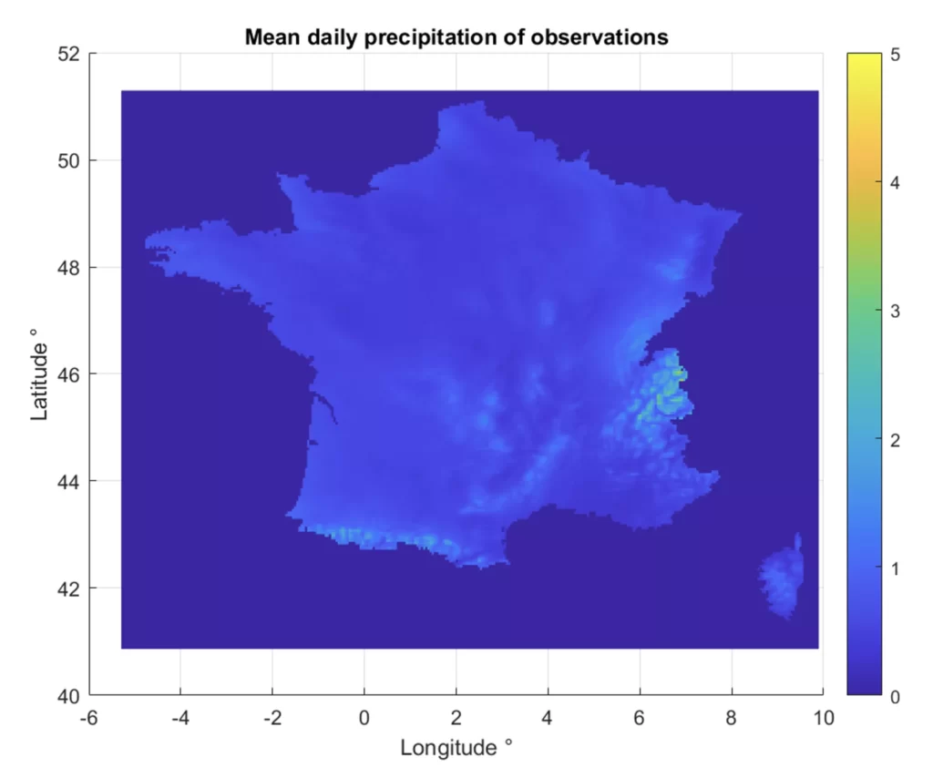
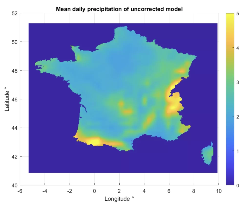
Let’s take the example of a climate model that overestimates mean daily precipitation in France (Figures 1 and 2).
The quantile mapping method is expressed as follows:

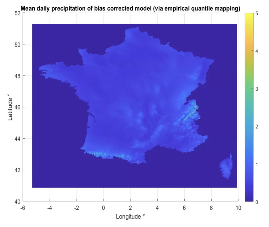
The climate model simulations for the future period are corrected with the distribution of observations from the reference period. We then obtain corrected climate simulations close to the observations (Figures 1 and 3), with differences in mean values close to 0.
Bias correction methods can be combined with downscaling approaches.


