What is statistical and dynamical downscaling?
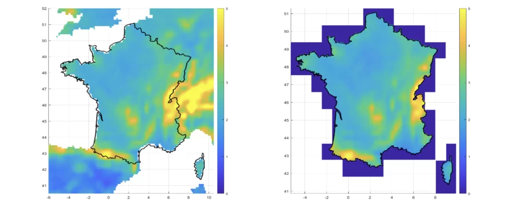
Climate models are essential tools for assessing the impact of greenhouse gas concentrations on changes in temperature and precipitation. However, their native spatial resolution is too coarse (~ 100 km) to represent regional and local phenomena in varied topography.
The so-called downscaling methods are needed to generate relevant climate information at the local scale, in terms of mean climate, main characteristics of variability, and extreme precipitation regimes. There are two approaches to downscale climate model simulations: statistical and dynamical downscaling.
For dynamical downscaling, higher resolution climate models are used. These models, known as regional climate models, use the lower-resolution climate models as boundary conditions and the principles of physics to reproduce the climate over a reduced area. As these models require a great deal of computing time, increasing the spatial and temporal resolution also increases computing time drastically, but enables a high degree of physical consistency to be maintained at the spatial level.
Statistical downscaling relies on statistical methods to statistically reduce the resolution of climate models. A range of statistical downscaling methods have been developed in recent years. The availability of local meteorological data is essential for statistical downscaling. The results of statistical downscaling become better when the observed historical weather data is of good quality over a long period of time. Statistical downscaling is performed using observed data from weather stations or gridded data sets. A statistical relationship is developed between observed climate data and climate model data for the same historical period. Statistical downscaling methods are easy to implement, unlike dynamical downscaling methods, but do not allow consistency to be maintained.
Statistical downscaling involves three steps:
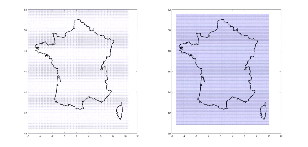
1. Mapping the raw climate model simulations to a common higher resolution grid corresponding to the resolution of the observations on which all the climate data will be scaled.

2. Interpolating each climate variable on the higher resolution reference grid. The interpolation method differs according to the climate variable; for example, a bilinear interpolation is generally used for temperatures, whereas a conservative interpolation of the modified Akima (makima) type is preferred for precipitation.

3. A bias correction method to compensate for systematic errors in raw data of climate models compared to observations.